The Matrix Preview tab allows you to visualize an in progress matrix.
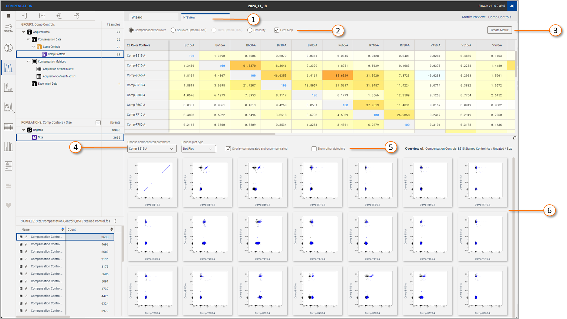
While creating a matrix, the preview tab can be clicked at any time to visualize the matrix that would be created with the current selections. You may toggle back and forth between Edit and Preview. Figure 1, element 1, indicates the control tabs.

Figure 1 Matrix Preview tab
| No. | Component |
|---|---|
| 1 | Wizard / Preview tabs |
| 2 | Matrix display options |
| 3 | Create matrix button |
| 4 | Preview plots display options |
| 5 | Show additional detectors |
| 6 | Preview plots |
Controls
Element 2 in Figure 1 controls what type of information is displayed about the selected matrix. Each option is described in detail below. Use the hierarchy to switch between any completed matrix to view or edit it.
NOTE: To retain the values of an in-progress matrix you must click the Create Matrix button.
Element 6 in Figure 1 is a preview of a selected sample + population combination, with the currently selected matrix applied. You may control which sample and population are being displayed using the hierarchy. In Figure 1, the population 'Size' is being previewed for the compensation control at the top of the sample list. Text on the upper righthand side of the preview window will confirm that sample and population. The preview will display one parameter at a time, versus all other parameters. We have chosen to abandon the all-by-all approach of previous FlowJo versions in favor of a set of graphs that are much more readable, paired with fluid controls. You may choose the type of plot and whether to show the uncompensated / raw overlay on each plot. Element 5 is a checkbox that allows you to visualize detectors that were not assigned as the primary detector for any fluorochrome, so that you may visualize the spillover across any detector pairing.
Matrix display options
Spillover Matrix
The default matrix displayed is the spillover matrix, which displays for each fluorochrome (row) the portion of the signal collected in each detector (column), normalized to the largest value which will display 1.00. A heatmap can be applied to this matrix that colors small values with light colors that get increasingly dark as they approach 1.00. Importantly, there is no value in the matrix that is abjectly 'wrong'. Larger values imply that a strong signal from a fluorochrome with likely a wide distribution was collected in more than one detector, but this can be unmixed and worked with. With spectral cytometry it is even likely with the denser arrangement of detectors that some adjacent detectors will have similar signals. This situation does imply that there is room to improve the panel design to reduce spillover spreading and make the data easier to analyze.
Spillover Spreading Matrix (SSM)
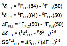
Choosing the second option, the SSM, will display a matrix that is more useful for assessing how good that panel is. The spillover spreading values are calculated for a given detector/spillover-color pair and can be calculated empirically by taking the square root of differences in squared robust standard deviations of measured fluorescence intensity from unstained negative and singly stained positive control populations:

Figure 2 SSM equations
Where:
- R stands for ‘Reference’, meaning the FL2- population in this example
- S stands for ‘Stained’, meaning the FL2+ population in this example
- Sigma is standard deviation (adjusted to use 84th and 50th percentile)
- F is fluorescence in units of intensity
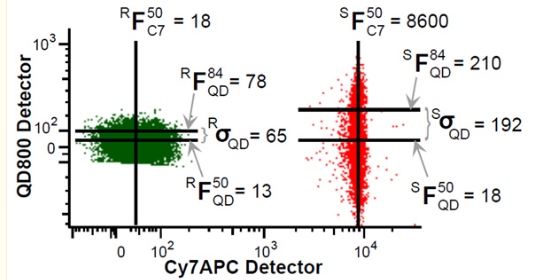
Here is a graphical example of those measures from Nguyen et. al.1

Figure 3 Graphical example of the SSM calculation
Unlike the spillover matrix, there are good rules of thumb regarding how good a combination is. SSM values under 5 indicate a pair of parameters will work will together. Values above 5 will grow increasingly difficult to work with until pairs of parameters with double-digit SSM values will be largely unusable. The SSM can be heat mapped, and the coloring will reflected this description, saturating bright read at 10.
Total Spread Matrix (TSM)
Looking at the equations used to calculate SSM, we can observe that the denominator in the calculation is the difference in median intensity (the 50th percentile) of the positive and negative population in the primary detector, which is essentially the stain index. This means a bright fluorochrome will have a smaller SSM value compared to a dim fluorochrome when they produce an equal amount of spread. This is generally acceptable as there are advantages to using bright fluorochromes, but if you would like to know the total spread introduced by a panel, regardless of brightness, you can view the TSM.
The TSM values can be heat mapped as well. This heatmap saturates at 2000, a value empirically determined to indicate a very poor pairing. Additionally, we note on the SSM matrix when there is a fluorochrome pair that produces a low (<5) SSM value but a high (>2000) TSM value to notify the user when significant spread is being masked by a bright fluorochrome.
Similarity
The similarity matrix displays the cosine similarity between a pair of fluorochromes. Cosine similarity is a measure of how similar two fluorochromes are, considering all detectors. The idea is that for a given fluorochrome (row in the spillover matrix) the set of detector values (columns) can be thought of as a multi-dimensional vector, and plotted. As an example, consider a data set with just 2 detectors. The spillover values in these detectors can be thought of as the x and y coordinates of a point. Draw a line from the origin (0,0) to that point and you have a vector describing the signal in all detectors for that fluorochrome. The angle that this line proceeds at can be described by its cosine. If you make this same calculation for two fluorochromes, the cosines can be compared and used as a metric of similarity. A value of 1.0 means that these fluorochromes are identical (and you will observe that the diagonal of the matrix which compares a fluor to itself, is 1.0), and smaller values indicate increasingly more different fluorochromes. The rule of thumb is that similarity values under ~0.93 are usable in a panel, but smaller is better and results will vary with instruments.
For more information on unmixing or compensation in FlowJo v11 see:
- Auto unmixing
- Compensation Wizard
