FlowJo v10 makes it easy to transform your raw data to expand or compress what is displayed on a graph.
The transform does not modify your actual recorded fluorescence data, only the amount of visual space that is allotted to various regions of the data. All digital (fcs3.0) data is output as linear and the options are for the software to log transform it (legacy) or biexponentially transform it (standard). One implementation of biexponential is called logicle as presented by Parks, Moore and Roederer (1).

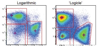
Why not simply view all data on a linear scale? The answer to that is the dynamic range of most flow data. “Positive” populations may be 10,000 times as bright as the “negative” populations, and thousands of bins wide, so we would need immense graphs to display most flow data in linear. Its much easier to visualize the positive populations if we compress the high intensity data into a smaller region with compact populations. The effect of log transformation is perfect for large intensity values, where clustering the data into discreet populations is most effective for accurate interpretation. However, the problem with a traditional log scale is evident as you approach lower intensity values and reach ‘0’.
At the low end of the intensity scale, we can expect some events to have zero or negative fluorescence values. This is because of 1) baseline correction by the instrument and 2) photon counting error which introduces a spread of measured intensity values due to inaccuracies in the photomultiplier tube (PMT). Therefore, a cell with near-zero intensity might report a negative value post-processing. Since zero and negative values cannot be displayed on a traditional log scale, all of these events will be allocated to the first bin and compressed onto the axis.
Furthermore, on a traditional log scale, the first and second decade only contain 10 divisions (or bins) for the data to fall into (bins 1 to 10) or ~90 bins (bins 11-100). Data at this end of the scale tends to be very disperse, due to the high resolution of these regions in the log scale. This dispersion can lead to visualization artifacts, which make it difficult to compare the populations effectively in this lower region to the populations with higher fluorescence intensity. The Herzenberg paper (review of logicle biexponential transformation) gives an excellent explanation of the transform and data display in general and we encourage anyone interested in the details of biexponential logicle transformation to read it!
FlowJo and Logicle
If the default settings are used in FlowJo, when digital data (fcs3.0) is brought into FlowJo it will be automatically biexponentially transformed using the logicle implementation. The fcs file does not contain any information as to the method of transformation. It is solely up to the software (e.g. FACSDiva, FlowJo, etc.) to scale it correctly.
For fcs3.0 data, uncompensated data will be transformed according to the Cytometers Preferences settings. Hence, you can change the preferences to change the transform on uncompensated data or to turn off the biexponential transform.
Once data is compensated, transforms are linked to the compensation matrix and will only adjust data that has the same compensation matrix applied. Different transforms can be applied to different files in the same workspace, if they have different compensation matrices.
With fcs2.0 data or ‘analog’ files, the transformation can be used on any compensated data, but there needs to be a compensation matrix associated with the file (hardware compensation done on analog instruments does not create a compensation matrix associated with the file). So the easiest way to allow for transformation on fcs 2.0 files is to collect them uncompensated and create the compensation matrix in FlowJo.
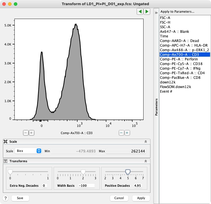
Once the data has been compensated, open a graph window and choose a compensated parameter to display on one or both axes. A small square button  will appear next to the axis label. Click this button to modify the display options.

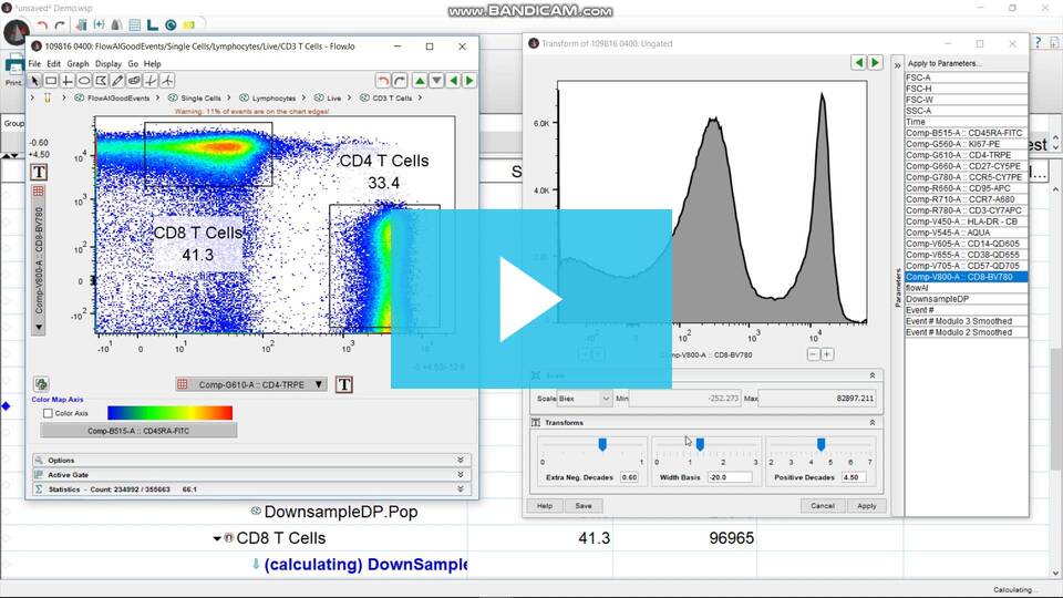
Here you can select between displaying linear, standard logarithmic display, or to customize the axis. Switching to log or linear immediately changes that axis to the selected scale. Clicking the Customize Axis option will cause a pop up window, as shown in the figure below, to appear that will let you modify the transform and the associated settings.

Bi-exponential Transforms:
The default display transformation process is called Biex and is based on a method developed by Dave Parks and Wayne Moore at Stanford University using a generalization of the bi-exponential function (1,2). The display functions approach true log for high data values and approach true linear around zero. This provides smooth, near-linear display of low and negative data values. It is implemented here through a lookup table for efficiency purposes.
The ArcSinh and Logicle transforms also transform data by passing it through functions that create a linear-like scale near zero and a log-like scale beyond an adjustable threshold, but importantly are implemented to produce results that match the published equations. Respectively, arcsinh and a scaled version of the sinh function are used(3). The equation based nature of these transforms makes it possible to create exact replicas of these transforms in other software, such as R.
Hyperlog is a log like function developed by Bruce Bagwell that approximates the log transform with a function that matches the log transform above zero, but has an inverse that can be used for ranges below zero (4). This transform is also implemented through an equation.
The Miltenyi transform that interpolates all negative and zero values to a -1 to 1 scale, and displays the rest of the data on a log scale. As the name implies, this equation was developed by the Miltenyi corporation and is most useful at reproducing acquisition displays from Miltenyi produced cytometers. This transform is implemented through a lookup table.
For a more detailed look at data transformations, please refer to the papers below:
References:
1) Herzenberg LA, Tung J, Moore WA, Herzenberg LA, Parks DR. Interpreting flow cytometry data: a guide for the perplexed. Nat Immunol. 2006 Jul;7(7):681-5.
2) James W. Tung, Kartoosh Heydari, Rabin Tirouvanziam, Bita Sahaf, David R. Parks, Leonard A. Herzenberg, Leonore A. Herzenberg. Modern Flow Cytometry: A Practical Approach. Clinics in Laboratory Medicine, Volume 27, Issue 3, Pages 453-468.
3) David R. Parks, Mario Roederer, Wayne A. Moore. A new “Logicle” display method avoids deceptive effects of logarithmic scaling for low signals and compensated data. Cytometry Part A, Volume 69A, Issue 6, pages 541-551, June 2006.
4) C. Bruce Bagwell. Hyperlog – A flexible log-like transform for negative, zero, and positive valued data. Cytometry part A, Volume 64A, Issue 1, pages 34-42, March 2005.
See More:
Display Transformation and Digital Data
Why Biexponential Transformation?

