Univariate modeling can be used to create a fit to cell cycle data based on statistics in one dimension, traditionally DNA content.
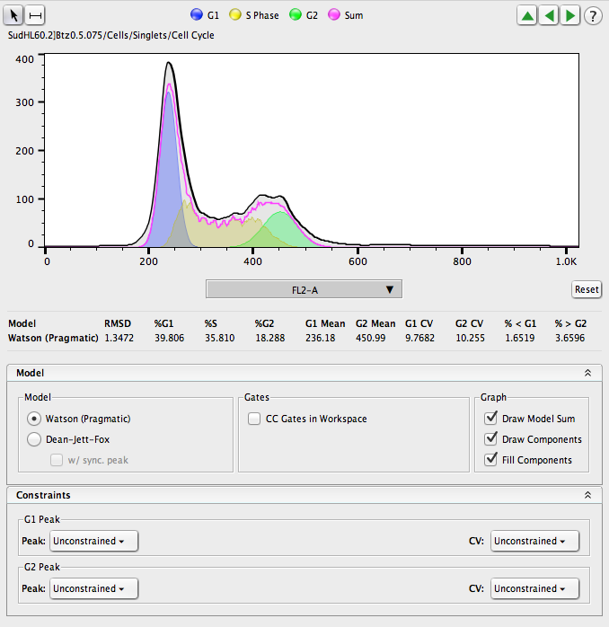
FlowJo provides a simple interface to performing fairly sophisticated DNA/Cell Cycle analysis. To launch the univariate cell cycle model click on the population of interest in the workspace, then select the Cell Cycle task from the Biology Band. The univariate model will appear by default as shown in Figure 1.

Figure 1
The Univariate Models
FlowJo v10 provides two univariate cell cycle platforms, the Watson Pragmatic algorithm (1) and Dean Jett Fox (DJF) (2). The two models differ in their mathematical calculations of each phase of the cell cycle. Consequently, results from one model may vary quite significantly from the other. It is good laboratory practice to consistently use the same model throughout a study when reporting or publishing statistics. The methods the models employ to calculate their statistics are described below.
Watson Pragmatic
The Watson model was published by James Watson and colleagues in 1987. It assumes only that the data within the G0/G1 and G2/M peaks are normally distributed and that one of those two peaks is identifiable. [3]
The model initializes by approximating G0/G1 peak as a Gaussian distribution and making an initial guess of the mean by finding the channel with the most cell in the left portion of the data. The standard deviation (SD) or width of the population is then approximated by finding the width of the distribution at 60% of the maximum height. A minimization process (least squares fitting) is then executed over a range of -3 to 1 standard deviations about the first guess mean to improve the fit. The range is unbalanced to the left since little data is expected to occur below the G0/G1 peak, while the S phase cells are expected to occur to the right and are more likely to overlap and skew the fit.
Once the G0/G1 peak is fit, the G2/M mean is placed at 1.75 x the intensity of the G0/G1 mean. Theoretically the G2/M peak will have a mean twice as bright as the G0/G1, but in practice there is some loss in the process and the G2/M peak ends up being not quite twice as bright.
The width is estimated in the same manner and a second Gaussian distribution is fit to the data using the same minimization process.
Dean-Jett-Fox
The Dean-Jett Fox (DJF) model is a modification to one of the original algorithms published for modeling cell cycle data, the Dean-Jett (3), and was published in 1980 in Cytometry.
The G0/G1 and G2/M curves are fit using the same process as the Watson model. The difference occurs in the fit of the S phase. The Dean-Jett model fit a second order polynomial (f (x) = Ax^2 + Bx + C) to the S phase. The Fox modification is to make the fit the addition of a Gaussian distribution and the polynomial. This modification gives the DJF model the ability to properly fit a synchronous population with a complex S phase distribution.
The ability to model a synchronous S-phase is included as an optional component in the user interface.
More details regarding the univariate statistics are available in the univariate statistics link.
Constraints
If the data fits the models default assumptions of a large identifiableG0/G1 peak, a smaller but identifiable G2/M peak, and little noise, the modeling process will generally create a credible result with no further effort. However, if the data does not match the default assumptions, you can constrain the coefficients of variation (CV) for each peak, the peak means, the ratio of the mean peaks, or any combination thereof.
Constraints on the variation
There are two options for constraining the CVs of the G0/G1 and/or G2/M populations. These can be found under the Constraints panel in the Cell cycle graphical user interface.
The first option allows the user to set the CV value manually “= n”. Simply select “= n” from the drop down menu and enter a value in the box. Hit “Enter” on the keyboard to view the effect of the change.
The second option allows the user to set one peak’s CV to that of the other. Select “= G1 CV” or “= G2 CV” to apply the constraints.
Constraints on the mean
The mean locations of the G0/G1 and G2/M peaks can be constrained relative to each other or within a specified range.
Relative constraints are based on the knowledge that G2/M cells have twice the DNA content of G0/G1 cells, though the detected intensity signal usually reflects a little more loss at the upper end producing a ratio just under 2. When setting the G2 peak relative to G1, select “= G1 x n” and enter a value near 2 (since G2 cells should have roughly twice the amount of DNA that G1 has). If you wish to set the G1 peak relative to G2, select “= G2 x n” and enter a value around 0.5 (Since cells in G1 should have roughly half G2’s DNA).
Selecting the “=G2 x” will force the ratio of the G2/M to G0/G1 peaks to be whatever number is entered. Try 1.95 as an initial guess if using this tool. Try additional values and see if the Root Mean Square (RMS) error improves with the changes. RMS is a measure of the distance between your model and the actual data, so smaller values are better. Because of the tremendous amount of variability in experimental conditions, there is not a specific RMS value that is deemed to be too large.
Batching the Model
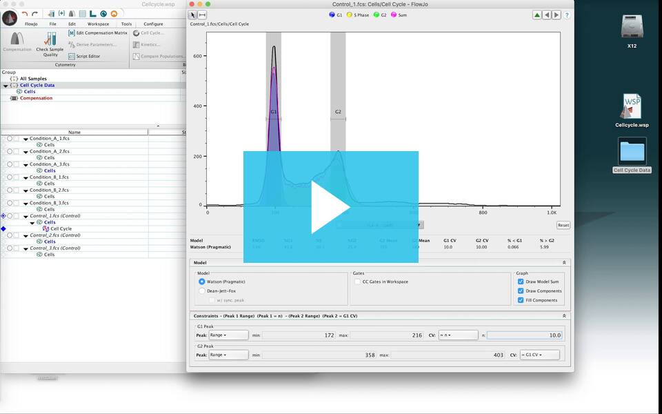
A Cell Cycle model, like any other node in FlowJo, can be applied to one or more samples either by dragging and dropping the node to other files or to the group. This process is explained on our copying gates page. If the model you create is unconstrained and then applied to multiple samples, FlowJo will create the best fit possible for all samples, unique to each sample. If you apply a constraint to the original file, that constraint will be applied to all other files that you drag the Cell Cycle model to. As an example, if you have an easy to model control file, you could create range gates around the obvious primary peaks. The constraint will have no effect on the model of the control, but if you apply this model to an experimental file in which the peaks are difficult to identify, the constraint will force the model to place the peaks in the same position as the control.
Creating Tabular or Graphical Outputs
Once models have been created for all files of interest, a table of statistics can be created for all files by dragging the cell cycle node to the table editor. Dragging in the node and batching will produce a table of all statistics for all files within the selected group. Individual statistics can be removed by clicking on the statistic in the table editor pre-batching, and clicking delete on your keyboard. See the univariate statistics page for a description of all the statistics used in this model.
Dragging the cell cycle node to a page in the layout editor produces the graphic from the cell cycle platform with the statistics overlaid. This graphic is then batchable if the model has been applied to all of the files in the desired group.
Citations:
1. Watson, Chambers, & Smith. A pragmatic approach to the analysis of DNA histograms with a definable G1 peak. Cytometry 8:1-8 (1987).
2. Fox, MH. A Model for the Computer Analysis of Synchronous DNA Distribution. Cytometry 1(1):71-77 (1980).
3. Dean PN, Jett JH. Mathematical analysis of DNA distributions from flow microfluorometry. J Cell Biol 60:523-527 (1974).
For more information see the relate links listed below:
Protocol for DNA / Cell Cycle using PI and BRDU
List of References about DNA dyes and analysis
Tags: FlowJo

