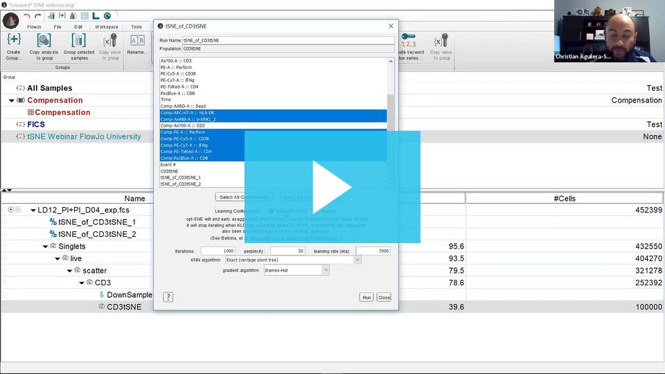
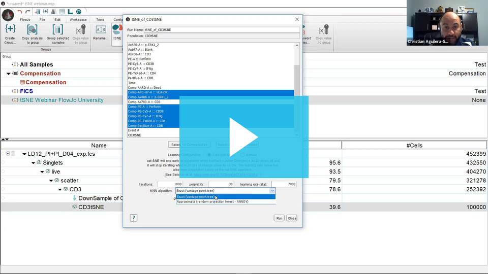
T-Distributed Stochastic Neighbor Embedding (tSNE) is an algorithm for performing dimensionality reduction, allowing visualization of complex multi-dimensional data in fewer dimensions while still maintaining the structure of the data.
tSNE is an unsupervised nonlinear dimensionality reduction algorithm useful for visualizing high dimensional flow or mass cytometry data sets in a dimension-reduced data space. The tSNE platform computes two new derived parameters from a user defined selection of cytometric parameters. The tSNE-generated parameters are optimized in such a way that observations/data points which were close to one another in the raw high dimensional data are close in the reduced data space. Importantly, tSNE can be used as a piece of many different workflows. It can be used independently to visualize an entire data file in an exploratory manner, as a preprocessing step in anticipation of clustering, or in other related workflows. Please see the references section for more details on the tSNE algorithm and its potential applications [1,2].
FlowJo v10 has an extremely powerful native platform for running tSNE. It can be accessed and run through the Populations menu (Workspace tab –> Populations band).
- The native platforms in FlowJo (such as tSNE) do not require R.
Video de tSNE en español
Practical Considerations
While tSNE is a powerful visualization technique, running the algorithm is computationally expensive, and the output is sensitive to the input data. This section will briefly cover a few key points in the area of preparing your data.
- Cleaning up your data – The best analyses begin with cleaning up raw data to exclude doublets, debris, and dead cells. This step reduces noise in the data and can improve the tSNE algorithm output. In addition, gate to include only the cells of interest (e.g., gating on CD3+ if T cells are of primary interest).
- Parameter Selection – In addition to choosing which events to use in your tSNE calculation it is also important to choose appropriate parameters. If your data set is fluorescence-based, select only compensated parameters (Comp-Parameter::Stain Reagent). Do not include parameters that may have been collected, but were not utilized in the staining panel and leave out any common parameters that do not vary across the sample population you are investigating. Inclusion of irrelevant parameters can add background noise in the calculation without contributing to the signal.
- Data Scaling – The tSNE algorithm operates on data as transformed within your workspace. Therefore, you may see an improvement in your results if your data is on scale and whitespace is minimized. For more information on this subject, see our help pages on transformations in FlowJo v10.
- Workflow- Because tSNE relies on the initial state of events seeded into the algorithm, the output will not be identical for different samples. One approach for comparing multiple samples is to concatenate all samples together and run tSNE on this single large file. You can either create a new keyword-based parameter denoting disease state, treatment group, or study arm, and add it to the concatenated file during the concatenation process, or use the SampleID keyword that FlowJo will automatically add to separate the files after running tSNE.
Creating tSNE Parameters
Basic Operation:
- Open FlowJo v10.5 or later.
- Select/highlight a sample or gated population node within the samples pane of the FlowJo workspace.
- Under the Populations menu (Workspace Tab –> Populations Band), select tSNE. This will bring up a Choose Selected Parameters window with options.
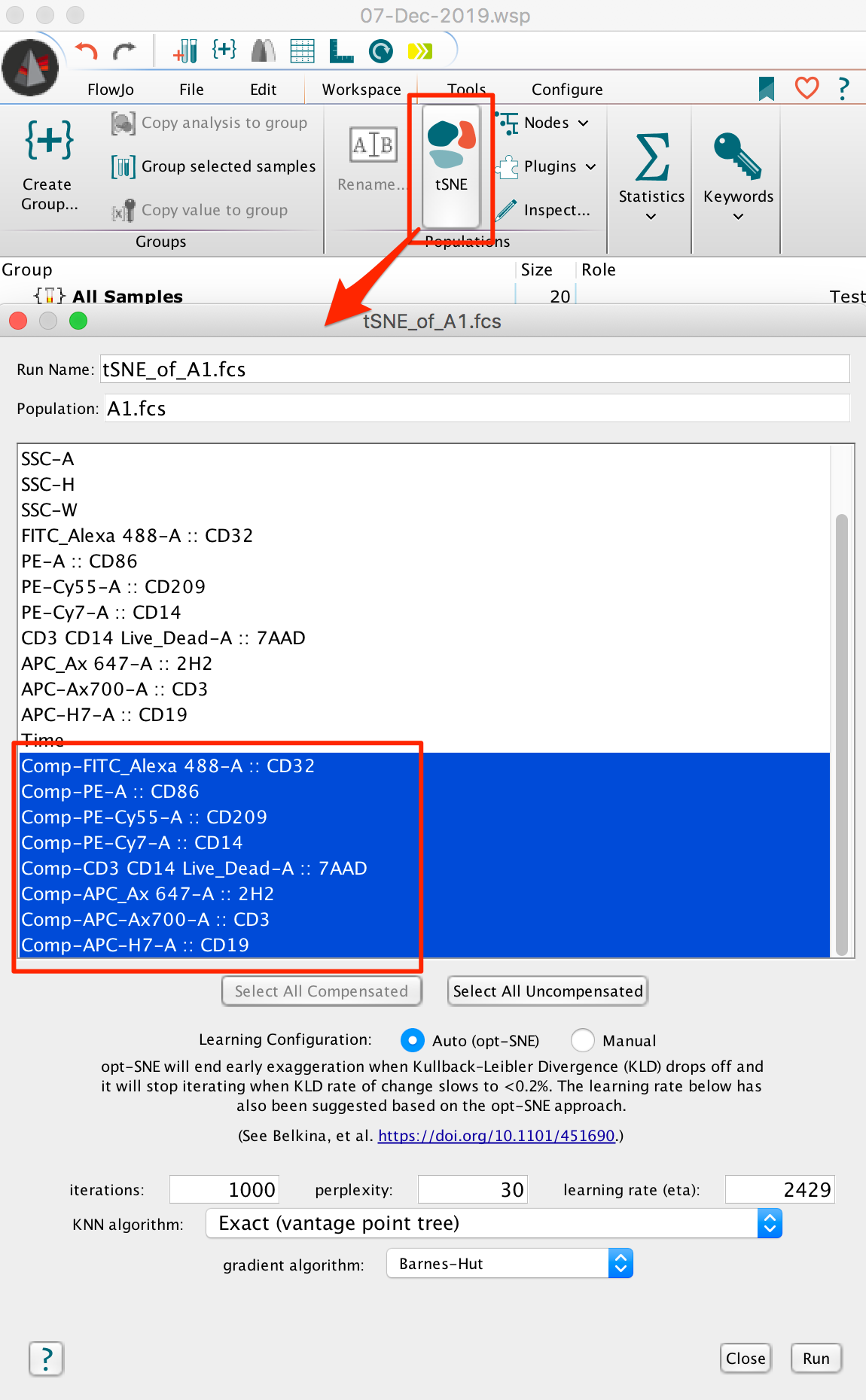
- Select the parameters to be used for the tSNE calculation. If your data is fluorescence-based, make sure to choose only compensated parameters (denoted by the Comp- prefix).
- Adjust settings (optional). Defaults have been provided as a starting point and should be acceptable for many data sets. The Opt-SNE algorithm utilized as an automated Learning Configurations is highly recommended (and selected by default). Opt-SNE will use the value in the Iterations setting as a maximum, and halt operation when the algorithm stops improving, saving you time.
- Initiate the calculation by pressing the “Run” button. The algorithm will run on the input population selected, utilizing selected options. The Platform will create two new parameters, which are the dimension-reduced outputs from the algorithm.
Technical Options:
Iterations – Maximum number of iterations the algorithm will run. A value of 300-3000 can be specified.
Perplexity – Perplexity is related to the number of nearest neighbors that is used in learning algorithms. In tSNE, the perplexity may be viewed as a knob that sets the number of effective nearest neighbors. The most appropriate value depends on the density of your data. Generally a larger / denser dataset requires a larger perplexity. A value of 2-100 can be specified.
Eta (learning rate) – The learning rate (Eta), which controls how much the weights are adjusted at each update. In tSNE, it is a step size of gradient descent update to get minimum probability difference. A value of 2-2000 can be specified. Optimally set at 7% the number of cells being mapped into tSNE space.
KNN algorithm – Sets the k nearest neighbors algorithm. One of the initial steps in tSNE is to calculate the ‘distance’ or similarity between pairs of cells, using the intensity values of all selected parameters. There are two options, a vantage point tree which is an exact method that calculates all distance between all cells and compares them to a threshold to see if they are neighbors, or the ANNOY algorithm, which is an approximation relying on not necessarily needing all of the nearest neighbors to significantly speed up the calculation.
Gradient algorithm – iterative adjustment to the embedding that maps high-dimensional data to a low-dimensional space is done by a gradient decent algorithm. The Barnes-Hut algorithm is the original implementation in FlowJo. The FFT (Fast Fourier Transform) interpolation is a more recent option that speeds up the process.
Visualizing the tSNE data space
The Graph Window
When the tSNE calculation on a sample is complete, new tSNE parameters will become available within the drop down parameter list of the graph window. The tSNE parameters can be used in any graphic, gating, or other analysis, as can any of the original sample parameters.
- Double click on the gated population used to calculate tSNE. This will open a graph window. Select TSNE_X vs TSNE_Y to view the reduced data space in the same orientation as the Create tSNE Parameters window displayed during the calculation.
- This will illustrate an “embedded” tSNE mapping of the data being illustrated. Islands within the tSNE space represent major populations within any population.
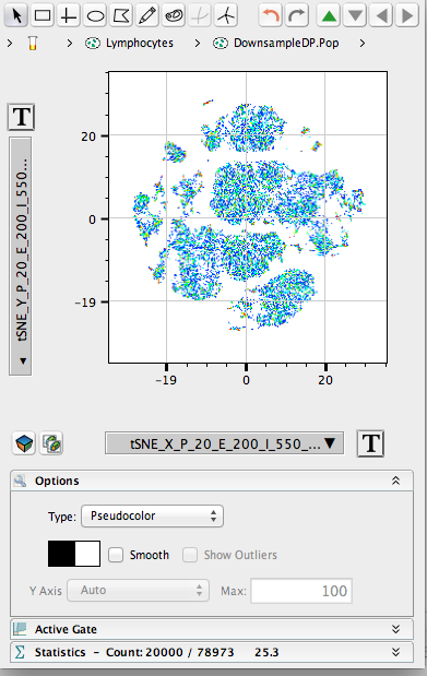
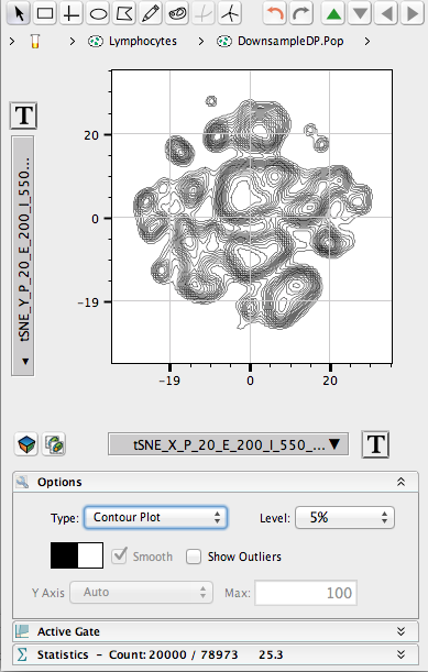
- This will illustrate an “embedded” tSNE mapping of the data being illustrated. Islands within the tSNE space represent major populations within any population.
The Layout Editor
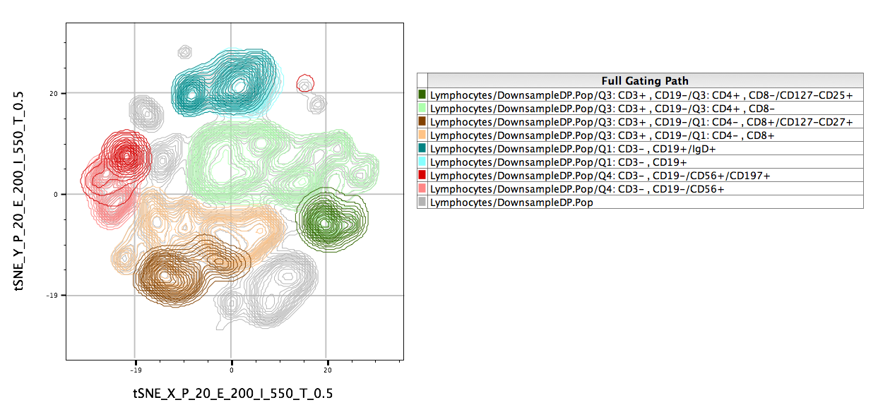
Overlays of gated populations can be displayed in the tSNE space using overlays within the Layout Editor. In the example below, we have taken the original population of interest and overlaid manually gated subsets. Note the distinct separation of markers in different regions of the map:
References.
1. Maaten and Hinton (2008). “Visualizing data using t-SNE.” Journal of Machine Learning Research, 9: 2579–2605.
2. Wallach, I.; Liliean, R. (2009). “The Protein-Small-Molecule Database, A Non-Redundant Structural Resource for the Analysis of Protein-Ligand Binding”. Bioinformatics 25 (5): 615–620.
Questions about tSNE? Send us an email at flowjo@bd.com

