Introduction
The Tracking Responders Expanding (T-REX) algorithm has been implemented as a FlowJo plugin. The T-REX algorithm creates a pair of dimensionality reduction parameters, identifies the areas of difference between two user specified conditions, clusters the data, then identifies the clusters that match the region of difference.
The T-REX FlowJo plugin is designed to be run on a single FCS file that contains two gates identifying events that were processed under different experimental conditions. Such an FCS file can be created by concatenating two or more individual FCS files, and adding a keyword-based parameter that defines which samples belong to a given experimental condition. Please refer to this documentation page on concatenation for more details: https://docs.flowjo.com/flowjo/workspaces-and-samples/samples-andfile-types/ws-export/
The plugin will create 4 new derived parameters added to the selected file in the FlowJo workspace – two dimensionality reduction parameters, one cluster results parameter, and one parameter that measures difference between conditions, along with gated cluster populations if differences are identified. Additional results files produced by the algorithm will be found within a TRex output_files folder within the derived parameters folder for the workspace in which the plugin was run.
Download and Installation
1. Place the plugin.jar file in your Plugins folder, and direct FlowJo to that folder using the Diagnostics section of the Preferences.
2. Make sure you have R installed and the R path is specified in the R Path field of the Diagnostics
section of the Preferences.
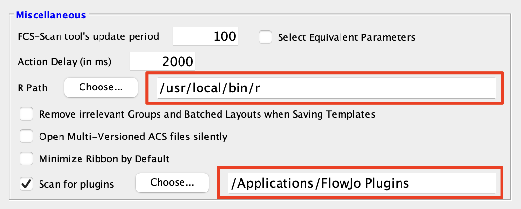
3. Restart the FlowJo application to pick up the new plugin.
Note: Running the T-REX plugin for the first time will install the R package dependencies required to run the T-REX algorithm into your R library. To install manually, type (or copy/pasting) the following in your R console:
install.packages(c(‘tidyverse’,’ggplot2′,’cowplot’,’FNN’,’dbscan’,’fancycut’,’gridExtra’,’uwot’,’RColorBrewer’,’dplyr’,’purrr’,’Rtsne’,’BiocManager’))
BiocManager::install(c(‘cytoMEM’,’flowCore’,’Biobase’))
For older versions of R, please refer to the appropriate Bioconductor release: https://bioconductor.org/about/release-announcements/
Additional documentation on installing plugins in FlowJo can be found here:
http://docs.flowjo.com/d2/plugins/installing-plugins.
Usage
To run the T-rex plugin on your FCS file:
1. Select a sample of interest with 2 gates identifying 2 populations to compare within the workspace.
2. Go to the Workspace tab and select the TRex option from within the Plugins dropdown menu
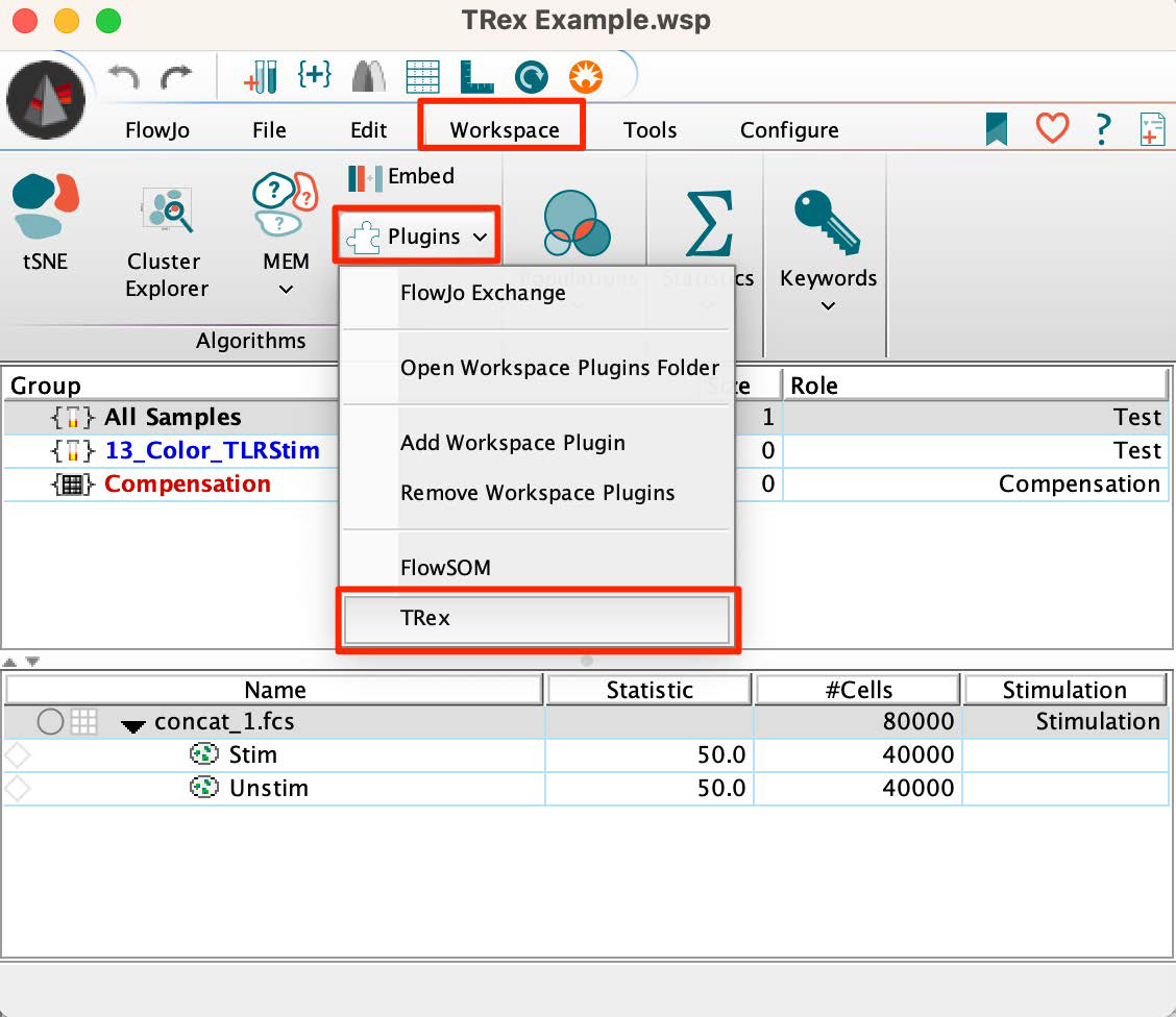 3. This dialog will appear:
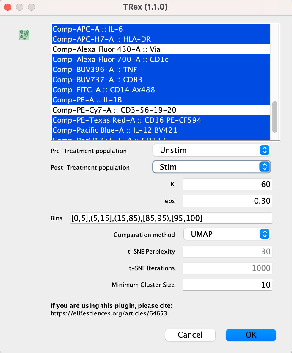
In the top box you must select the parameters for the algorithm to consider. In general, select any parameter that may have differentiating power between the groups. In this example, the live/dead and dump channels have been omitted as those parameters were employed for gating during pre-processing. The top two selection boxes must be used to select the two populations to compare, using gates as the method for identifying cells of each type.
Other options include:
• K – The number of nearest neighbors to consider during clustering.
• eps – The radius of the epsilon neighborhood. Two points are considered neighbors if the distance between them is below the threshold epsilon.
• Bins – The percentage of cells from one condition to be highlighted.
• Comparison method – UMAP or tSNE
• t-SNE perplexity – Size of the neighborhood setting, exclusively for the tSNE choice.
• t-SNE iterations – Set a maximum limit on tSNE iterations.
• Minimum Cluster Size – Minimum number of events to be considered a cluster
The results will be four derived parameters: two trex_DRmethod parameters representing the low dimensional embedding results using the selected dimensionality reduction method, a trex_percent_change parameter (a measure of the representation of each class across the dimensionality reduction space), and a trex_cluster parameter for identifying clusters.
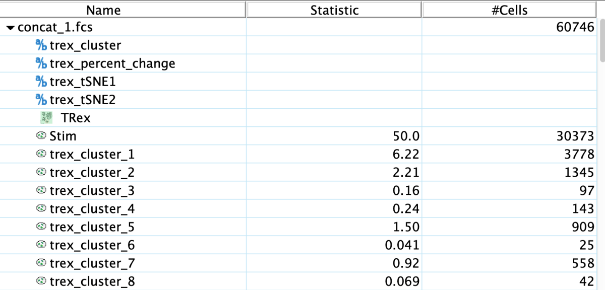
Plotting this outcome using the tSNE parameters and heat mapping by tex_percent_change, then juxtaposing it with a heat map of parameter expression can provide an understanding of the data and where it varies between conditions.
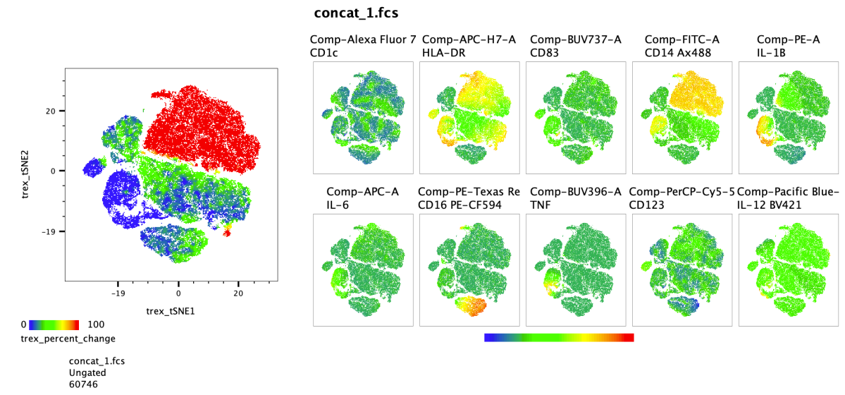
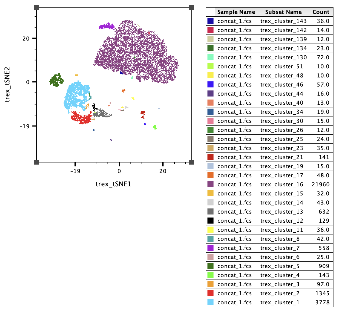
In this example we can see that the unstimulated cells for a population that is largely unique from the stimulated cells, appearing bright red in the plot. And likewise, the stimulated cells for a couple unique blue populations. The cluster results can also be viewed in FlowJo, perhaps most usefully as an overlay.
The plot below shows the clusters with differential power.
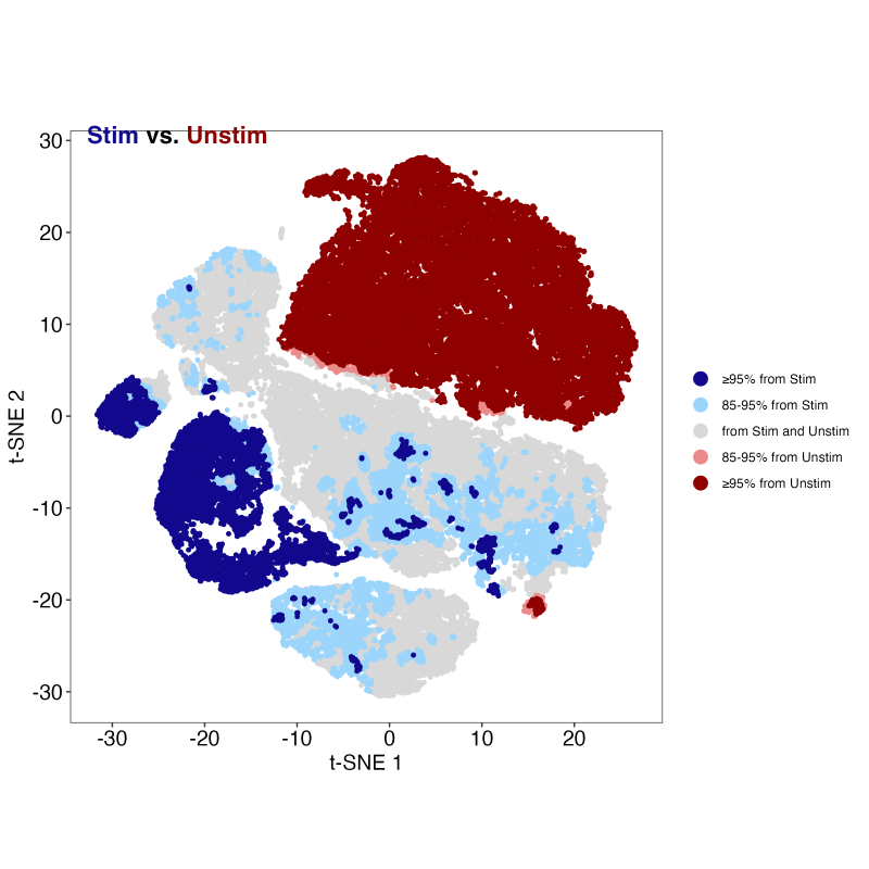
A number of useful plots are created in the TRex derivative folder as well. Perhaps the most informative is the blue-red cluster plot that shows which regions have significant expansion of one category or the other:
Leave us your feedback
Please write to flowjo@bd.com with any questions or concerns.
References
Sierra M Barone, Alberta GA Paul, Lyndsey M Muehling, Joanne A Lannigan, William W Kwok, Ronald B Turner, Judith A Woodfolk, Jonathan M Irish. Unsupervised machine learning reveals key immune cell subsets in COVID-19, rhinovirus infection, and cancer therapy.
